I’ve now written enough code for the PIC on the CatTrack base station such that I can begin to test it!
I’ve already tested comms with the CatTrack collar, using a development board instead of the base station. Read about that here.
Unfortunately, when testing my base station I found that it was nowhere near as sensitive as the development board – the base station was getting CRC errors whilst the development board was still receiving the signal fine. After a small bit of investigation I found out why. The problem is all down to the fact that I want to use the CC1125 at the lowest baud rate (300 bps), and consequently a very narrow receive bandwidth (3.8 kHz).
Before I get to the problem, we need to understand some theory. CatTrack uses a modulation scheme called Frequency Shift Keying (FSK). I am using a carrier frequency of 868 MHz and a frequency deviation of 1 kHz. This deviation is the value recommended by TI for a baud rate of 300 bps. This means that in order to transmit a ‘0’, the transmitter transmits a signal at (868 MHz – 1 kHz) for (1 / 300) seconds, so 867.999 MHz for 3.3 milliseconds. In order to transmit a ‘1’, the transmitter switches to (868 MHz + 1 kHz), so 868.001 MHz and sits there for 3.3 milliseconds. Bit by bit our entire message is transmitted. Makes sense right?
Carson’s bandwidth rule tells us the occupied bandwidth of the transmitted signal:

Where:
 is the bandwidth occupied by the signal
 is the frequency deviation
 is the modulating bit rate
An important thing to note here (and the source of much confusion in various forums!) is that is equal to the  in our case. Our highest baud rate will be when sending an alternating 0-1-0 sequence. As we saw above, this means we transmit for 3.3 milliseconds on one frequency, then 3.3 milliseconds on another. Thus the period is 6.6 milliseconds, therefore the bit rate is
  .
.
So in our case, the bandwidth occupied by the transmitted signal is:

Now, in the receiver we have a receive bandwidth of 3.8 kHz. The receive bandwidth needs to be set to a value such that the transmitted signal fits comfortably inside it.
In theory this sounds perfect – our receive bandwidth is 3.8 kHz and our transmitted signal only occupies 2.3 kHz, everything should work just fine!
However… this maths assumes that the transmitter transmits its signal centred exactly on 868 MHz, and that the receiver places its 3.8 kHz receive window exactly around 868 MHz. The reality is somewhat different.
We have frequency references inside our transmitter and receiver from which the transmit and receive frequencies are derived. These have an inherent accuracy, expressed in parts per million (ppm). A 1 MHz reference oscillator with an accuracy of ±10 ppm could in reality output any value from 0.99999 MHz to 1.00001 MHz. This doesn’t look too bad, but by the time this signal is multiplied up to our transmit frequency, using a reference oscillator with an accuracy of ±10 ppm means that instead of transmitting on exactly 868 MHz, we could be transmitting at 868.008680 MHz – as much as 8.7 kHz off the correct frequency! Remembering that our receive window is only 3.8 kHz, transmitting 8.7 kHz away from the correct frequency is a big problem – our receiver will never even see our transmitted signal!
The frequency reference components I’ve used in CatTrack are TG-5021CG Temperature Controlled Oscillators (TCXOs). Their specification is ±2 ppm. Better than ±10 ppm, but still a problem for us with our narrow receive bandwidth.
Taking the extreme (but plausible) example, where our transmitter TCXO is +2 ppm and our receiver TCXO is -2 ppm, we will end up in the following situation:
The lowest frequency in our transmitted signal will be at:

And the highest at:

Now, assuming the TCXO in our receiver comes from the factory at -2 ppm (still within the ±2ppm specification), our 3.8 kHz receive window will start at:

and end at:

And now given that a picture speaks a thousand words:
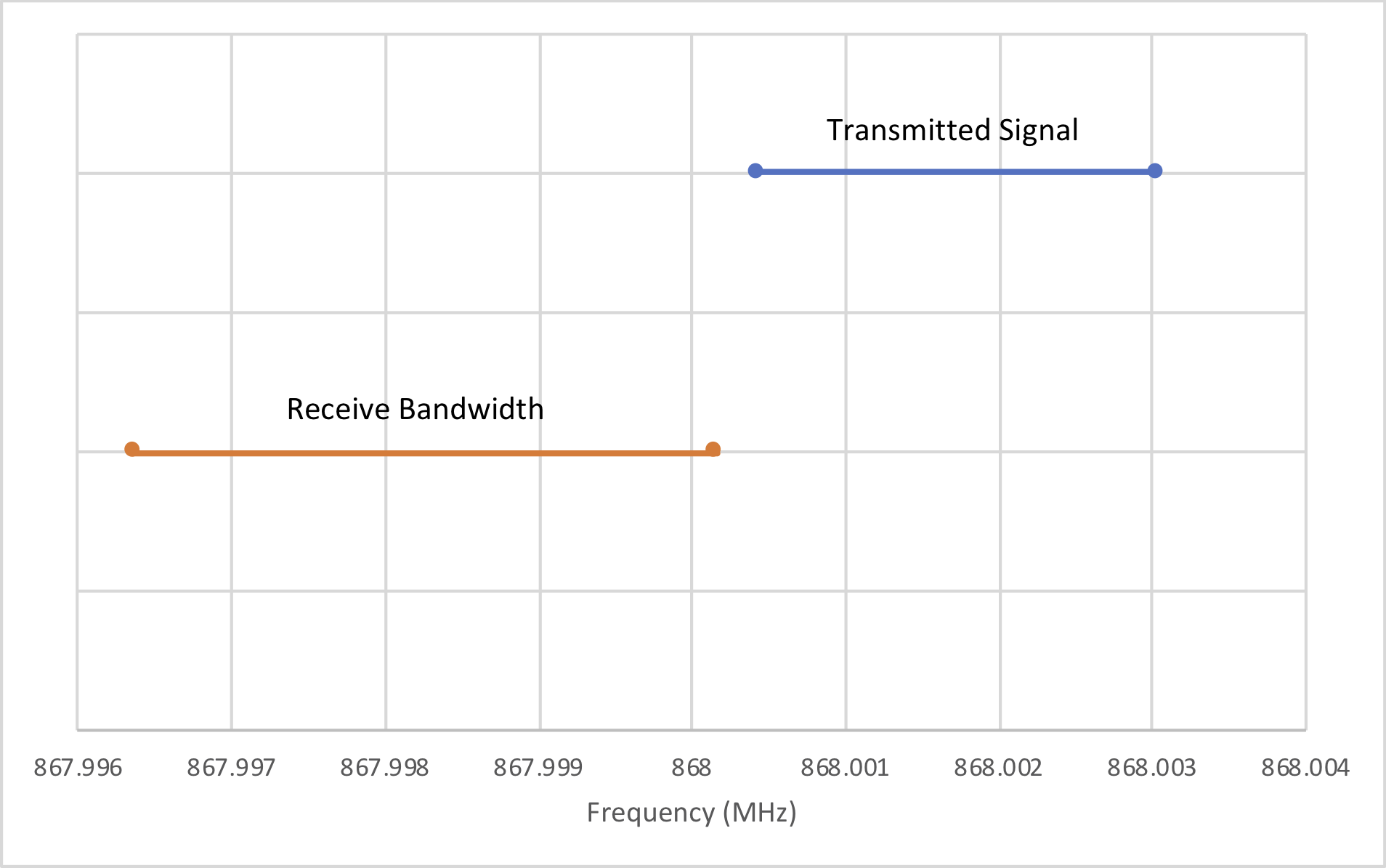
Our transmitted signal occupies the spectrum covered by the blue line and our receiver is listening in the region shown by the orange line (ignore the y-axis, they’ve only been spaced out for clarity).
Clearly this is bad and explains why our receiver isn’t properly receiving the signal that the collar is transmitting. But what can we do about it?
Thankfully there is something we can do, without putting more accurate frequency references in the transmitter and receiver (which would take more power, space and expense).
The CC1125 has a frequency offset feature whereby after receiving a packet, it populates a register with a value that represents the measured frequency offset between transmitter and receiver, thus:
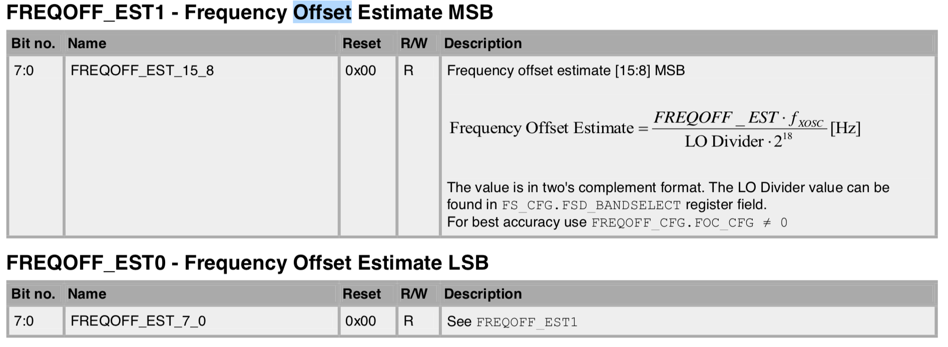
We can then program this calculated offset back into the FREQOFF registers, thereby shifting our receive window to match the transmitted signal. Magic!
In practice, the first thing we do is set our receiver to a larger receiver bandwidth by writing to the CHAN_BW register. I’m using 10 kHz. This is to be sure that we receive the transmitted signal so we can calculate the offset, like this:
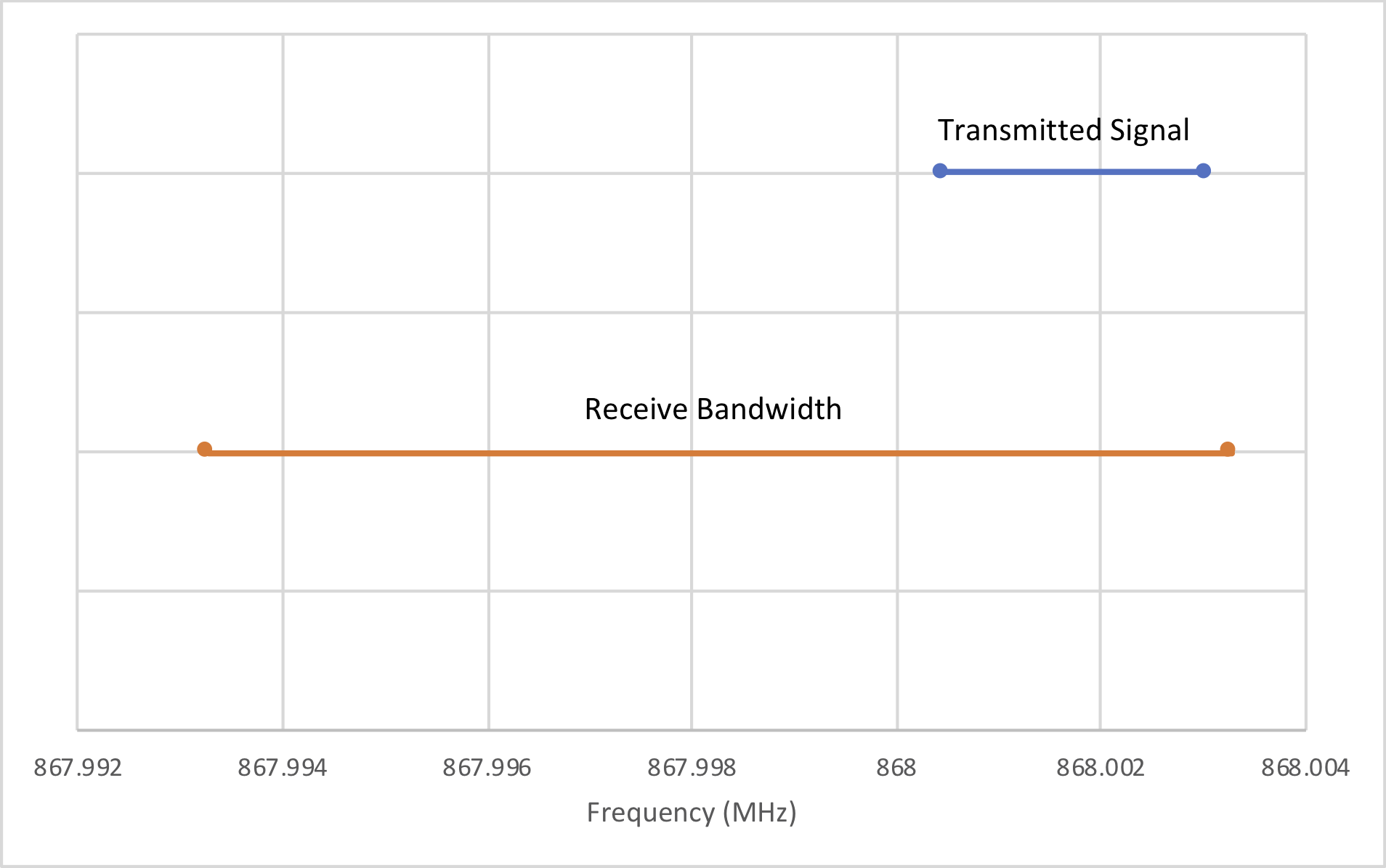
As we can see, the transmitted signal is now falling inside our receive bandwidth. Now we wait for a packet to arrive from the transmitter and as soon as it arrives we read back the FREQOFF_EST registers from the CC1125 and program them back into the FREQOFF register, shifting our receive window to match the transmitted signal. As a point of interest, you can alternatively send the SAFC strobe to automate this register reading/writing process.
Now that our receive window is aligned with our transmitter, we can take the receive bandwidth back down to the 3.8 kHz. This is how we end up:
![]()
Perfect! As soon as I had carried out this procedure I was measuring a receive sensitivity of -124 dBm and I was out-performing the development board.
This procedure is essential if you want to use the CC1125 for long-range communications. I thought I could get away with not doing it, but clearly the Maths shows that you do need it!
You may wonder why we don’t just simply leave the receive bandwidth set to 10 kHz and not bother with any of this offset setting malarky. The reason is down to receive sensitivity. Every time we half the receive bandwidth, we add 3 dB to our sensitivity. Therefore it stands that the narrower the receive bandwidth, the greater our range.
A couple of other things I did to the CC1125 to optimise it for long range communications:
- Set the FREQOFF_CFG register to 0x30 – this enables a feature called ‘frequency offset correction’. It’s explained well in the CC1125 manual, but the long and short of it is that it increases the effective receive bandwidth by BW/4, without compromising sensitivity.
- Change the modulation type from FSK to GFSK. GFSK is more bandwidth efficient than FSK, so you can get away with a slightly narrower receive bandwidth (Carson’s rule doesn’t properly apply to GFSK).
Interesting project – In testing what kind of range are you managing to get?
As I type this I’m tracking Buttons 170 metres away and I’m receiving the signal at -114 dBm. Given that I can receive signals down to around -126 dBm, I would expect several hundred metres to be easily achievable. One thing to bear in mind is that the range massively depends on the foliage/brick walls/etc. I’m tracking him from inside my house – even if I just go outside it’ll improve the range. Also when he climbs into a wet bush or lies on the tracker then the sensitivity can be reduced by up to 20 dB, massively reducing the range, but you would expect that he’d lift his head up at some point and you’d receive the signal.